Multiple regression prediction and estimation
Published:
This post covers Introduction to probability from Statistics for Engineers and Scientists by William Navidi.
Basic Ideas
- An Example
- A mobile ad hoc computer network consists of several computers (nodes) that move within a network area. Often messages are sent from one node to another. When the receiving node is out of range, the message must be sent to a nearby node, which then forwards it from node to node along a routing path toward its destination.
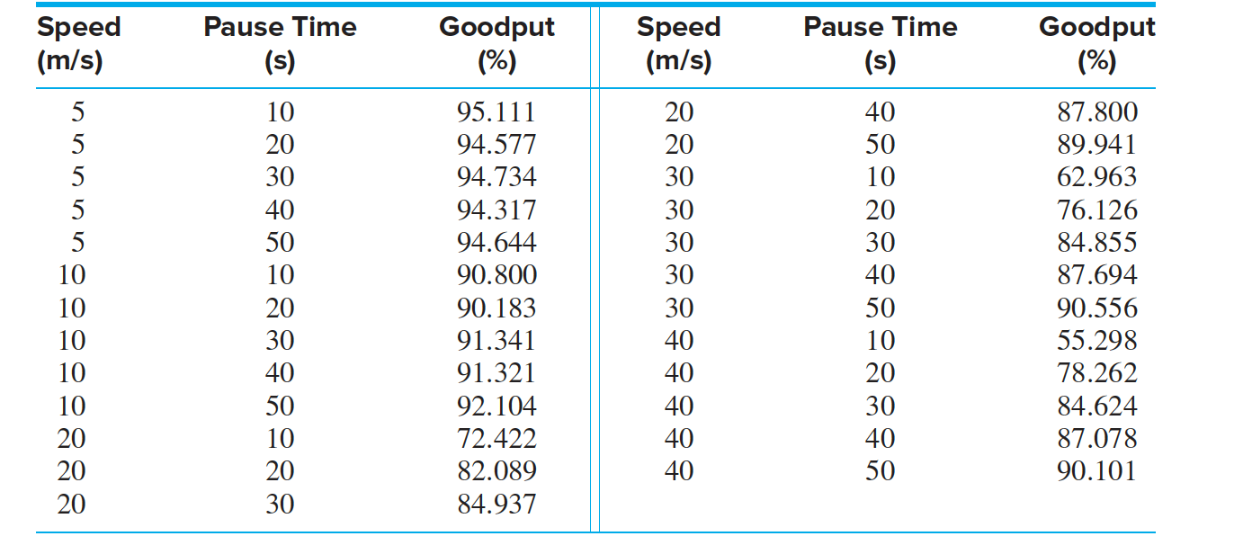
- We wish to predict the proportion of messages that will be successfully delivered, which is called the goodput.
- It is known that the goodput is affected by the average node speed and by the length of time that the nodes pause at each destination. Table presents average node speed, average pause time, and goodput for $25$ simulated mobile ad hoc networks.
Use the multiple regression model to predict the goodput for a network with speed $12$ m/s and pause time $25$ s.
For the goodput data, find the residual for the point Speed = $20$, Pause = $30$.
Find a $95\%$ confidence interval for the coefficient of Speed in the multiple regression
model.
Test the null hypothesis that the coefficient of Pause is less than or equal to $0.3$.
$Goodput = \beta_0 + \beta_1 Speed + \beta_2 Pause + \beta_3 Speed ⋅ Pause + \beta_4 Speed^2 + \beta_5 Pause^2 + \epsilon$
| Predictor | Coef | SE Coef | P |
|---|---|---|---|
| Constant | 96.024 | 3.946 | .000 |
| Speed | −1.8245 | 0.2376 | .000 |
| Pause | 0.5652 | 0.2256 | .022 |
| Speed*Pause | 0.024731 | 0.003249 | .000 |
| Speedˆ2 | 0.014020 | 0.004745 | .008 |
| Pauseˆ2 | -0.11793 | .003516 | .003 |
The regression equation is
$ Goodput = 96.0 − 1.82 Speed + 0.565 Pause + 0.0247 Speed*Pause + 0.0140 Speedˆ2 −0.0118 Pauseˆ2 $
Since there are $n = 25$ observations and $p = 5$ independent variables, the number of degrees of freedom for the Student’s t statistic is $25 − 5 − 1 = 19$.
The P-values for the tests are given in the next column. All the P-values are small, so it would be reasonable to conclude that each of the independent variables in the model is useful in predicting the goodput
- Analysis in multiple regression
- The predicted value $ \hat y$ is found by substituting $Speed = 20$ and $Pause = 30$ into the fitted model presented in the solution.
- The observed value of goodput is y = 84.937.
- This yields a predicted value for goodput of. $ \hat y = 86.350$.
- The residual is given by $y- \hat y = 84.937 − 86.350 = −1.413$.
$95\%$ confidence interval
From the output, the estimated coefficient is $−1.8245$, with a standard deviation of $0.2376$. To find a confidence interval, we use the Student’s t distribution with $19$ degrees of freedom. The degrees of freedom for the t statistic is equal to the degrees of freedom for error. The t value for a $95\%$ confidence interval is $t_{19, .025} = 2.093$.
The $95\%$ confidence interval is
$−1.8245 \pm (2.093)(0.2376) = −1.8245 \pm 0.4973 = (−2.3218, −1.3272)$
Test the null hypothesis
The estimated coefficient of Pause is $ \hat \beta_2 = 0.5652$, with standard deviation $ \hat s_ {\beta_2} = 0.2256$. The null hypothesis is $ \beta_2 ≤ 0.3$. Under $H_0$, we take $ \beta_2 = 0.3$, so the quantity
$t = \frac {\beta_2 − 0.3} {0.2256}$
has a Student’s t distribution with 19 degrees of freedom. Note that the degrees of freedom for the t statistic is equal to the degrees of freedom for error. The value of the t statistic is $(0.5652 − 0.3)∕0.2256 = 1.1755$. The P-value is between $0.10$ and
0.25. It is plausible that $ \beta_2 ≤ 0.3$.